Week 5 Lecture ML : Neural Net cost funcion

We're going to consider two types of classification problems.  The first is Binary classification, where the labels y are either 0 or 1.  In this case, we will have 1 output unit, so this Neural Network unit  on top has 4 output units, but if we had binary classification we would have only  one output unit that computes h(x).  And the output of the neural network would be h(x) is going to be a real number.  And in this case the number of output units,  S L, where L is again the index of the final layer.  Cuz that's the number of layers we have in the network so  the number of units we have in the output layer is going to be equal to 1.  In this case to simplify notation later, I'm also going to set K=1 so  you can think of K as also denoting the number of units in the output layer.  The second type of classification problem we'll consider will  be multi-class classification problem where we may have K distinct classes.  So our early example had this representation for y if we have 4 classes,  and in this case we will have capital K output units and  our hypothesis or output vectors that are K dimensional.  And the number of output units will be equal to K.  And usually we would have K greater than or equal to 3 in this case, because  if we had two causes, then we don't need to use the one verses all method.  We use the one verses all method only if we have K greater than or equals  V classes, so having only two classes we will need to use only one upper unit.  Now let's define the cost function for our neural network.

youtu.be/aircAruvnKk

잘 만듬 

 

 

Cost Function

Let's first define a few variables that we will need to use:

• L = total number of layers in the network
• s_lsl​ = number of units (not counting bias unit) in layer l
• K = number of output units/classes

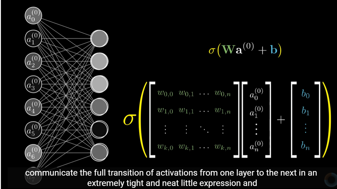
Recall that in neural networks, we may have many output nodes. We denote h_\Theta(x)_khΘ​(x)k​ as being a hypothesis that results in the k^{th}kth output. Our cost function for neural networks is going to be a generalization of the one we used for logistic regression. Recall that the cost function for regularized logistic regression was:

J(\theta) = - \frac{1}{m} \sum_{i=1}^m [ y^{(i)}\ \log (h_\theta (x^{(i)})) + (1 - y^{(i)})\ \log (1 - h_\theta(x^{(i)}))] + \frac{\lambda}{2m}\sum_{j=1}^n \theta_j^2J(θ)=−m1​∑i=1m​[y(i) log(hθ​(x(i)))+(1−y(i)) log(1−hθ​(x(i)))]+2mλ​∑j=1n​θj2​

For neural networks, it is going to be slightly more complicated:

J(Θ)=−1m∑i=1m∑k=1K[y(i)klog((hΘ(x(i)))k)+(1−y(i)k)log(1−(hΘ(x(i)))k)]+λ2m∑l=1L−1∑i=1sl∑j=1sl+1(Θ(l)j,i)2

We have added a few nested summations to account for our multiple output nodes. In the first part of the equation, before the square brackets, we have an additional nested summation that loops through the number of output nodes.

In the regularization part, after the square brackets, we must account for multiple theta matrices. The number of columns in our current theta matrix is equal to the number of nodes in our current layer (including the bias unit). The number of rows in our current theta matrix is equal to the number of nodes in the next layer (excluding the bias unit). As before with logistic regression, we square every term.

Note:

• the double sum simply adds up the logistic regression costs calculated for each cell in the output layer
• the triple sum simply adds up the squares of all the individual Θs in the entire network.
• the i in the triple sum does not refer to training example i

 

 

https://www.youtube.com/watch?v=Ilg3gGewQ5U